Saturated hydraulic conductivity: Double ring infiltrometer

Saturated hydraulic conductivity is one of the most important soil hydrophysical characteristics. Its determination is needed for many different applications and it is a key parameter for solutions in soil physics, hydrogeology, environmental protection, soil and groundwater protection against pollution, soil reclamation, irrigation and drainage for agricultural and non-agricultural purposes, landfill foundation, sport surfaces, etc.
It is also one of the main input parameters for models simulating transport of water and solutes through the soil profile.
The soils can be classified according to the scale described in Tab 1.




Tab 1. Soil classification table based on values of saturated hydraulic conductivity K (according to the formerly valid Czech standard
CSN 721020)

Soil (according the relative permeability)	Approximate range of saturated hydraulic conductivity (m s-1)	Examples of soil types
Highly impermeable	< 10-10	clays with low and medium plasticity, clays with high and extremely high plasticity
Impermeable	from 10-8 to 10-10	gravel loams, gravel clays and sandy clays, loams with low and medium plasticity
Lowly (poorly) permeable	from 10-6 to 10-8	sandy loams, loamy sands and clayey sands, loamy gravels and clayey gravels
Permeable	from 10-4 to 10-6	sands and gravels , containing fine-grained fraction (5 – 15 %)
Highly permeable	> 10-4	sands and gravels without or with very low fine grained fraction (<5%)

Double ring infiltrometer (Parr and Bertrand, 1960) The double ring infiltrometer is a widely used method of infiltration test used in many applications; i.e. design of land drainage pipes, design of sports surfaces, golf courses, isolation layers of the communal waste, etc. The infiltrometer consists of two concentric metal rings (see Fig 1), which are driven into the soil, and of a perforated metal plate. Equipment The double ring infiltrometer, wooden piece or something similar in order to drive the rings into the soil, hammer, bucket, measuring jug, scissors, knife, stopwatch, equipment for writing records, measuring tape, washcloth, and water.

Fig 1. Schema of the double ring infiltrometer.

Measurement procedure

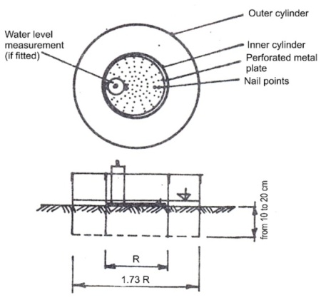
The measurement is taken in the inner cylinder; the outer cylinder is used only as a tool to ensure that water from the inner cylinder will flow downwards and not laterally. The soil surface in the inner cylinder is covered by a perforated metal plate which is used in order to dissipate the force of the applied water, to distribute water uniformly inside the ring and to prevent disturbance of the soil surface (see Fig 1).


Two nail points of different lengths are fixed to the metal plate. These nail points are used for observation of decreasing water level during the infiltration. Both (inner and outer) cylinders are driven into the soil (to a depth of 10-20 cm). It is recommended that the turf around the rings' periphery is cut with a knife, the soil is then less disturbed by driving the rings into it. The metal plate is placed on the soil surface in the inner cylinder, and water is poured into both cylinders (the water level in the inner cylinder should reach the upper nail point).


At this moment the stopwatch is started and the time needed for the water level to drop from the upper nail point to the lower nail point is measured and recorded. After this elapsed time, a certain amount of water was infiltrated (in this case 500 cm³). When the water level reaches the lower nail point, the time is recorded and the same amount of water is poured back from a prepared graduated bottle (500 cm³) (watch the video to see this procedure). The water level in the outer cylinder is kept at the same level as the water level in the inner cylinder.


Results from the double ring infiltrometer measurements can be taken only as directory information; however they can be considered as accurate enough for many applications.

DATA RECORD and CALCULATION from the double ring infiltrometer experiment

The measured data are recorded to a Data record form, like that on the right-hand side. This form includes the necessary parameters for our double-ring infiltrometer demonstrated in the video and the photos. However, these parameters can be different for other double ring infiltrometers. The measured data i(t) are then plotted into a graph (mm paper in the field or MS Excel) for the visual check of the measured data. The measured data are analysed based on the known Philip’s infiltration equations (Philip, 1957):

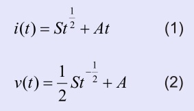where i(t) is cumulative infiltration, S is sorptivity, t is time and A is a parameter

The measurement provided values of i and t in the equation (1), the parameters S and A need to be determined, so the line described by equation (1) fits the measured points as well as possible. One of the widely used approximation methods, the method of the least squares, can be applied in order to find these unknown parameters A and S. When parameters A and S are known, infiltration rate v can be calculated for any given time according to the second of Philip’s equation (equation 2).
Steady-state infiltration rate after a longer time of infiltration (the line of the infiltration rate is parallel to the horizontal axis of time) remains constant and its value is close to the value of saturated hydraulic conductivity K. The following formula can be used:

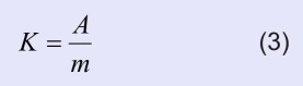where K is saturated hydraulic conductivity and m is a constant equal to 0.66667 (= 2/3)

The calculated value of K is then used for soil classification according to Tab. 1.

Example of data analysis

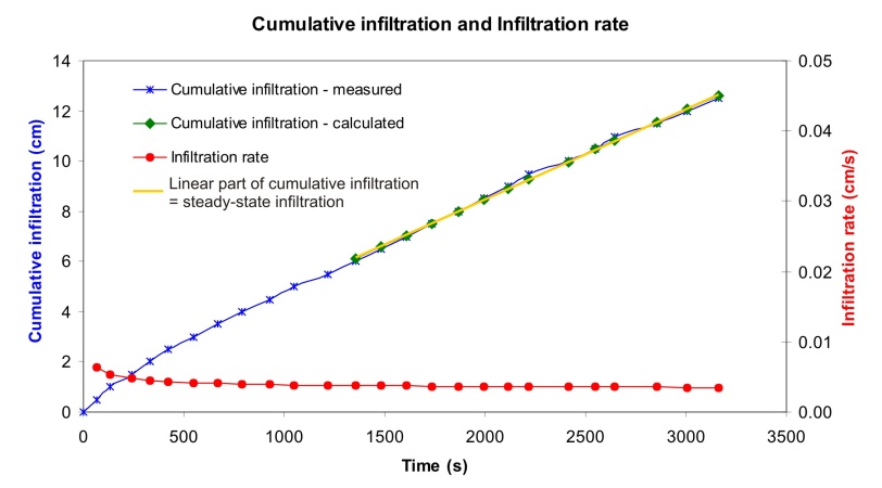
See the table to the right. The measured data need to be prepared first. A cumulative infiltration in bulk units needs to be recalculated by using an infiltration area to the height of cumulative infiltration in length units. Then, we plot a graph and find a linear part where the infiltration is steady-state (the yellow part of the table). The unknown parameters S and A from the equation (1) will be calculated from that linear part by using the least squares method. We can use the SOLVER function in MS Excel. (Find the Solver in Tools or activate it in Tools - Add-ons.) We have to find the best straight line to fit our measured linear part of data. This means the sum of squared residuals must be as small as possible.

We put a formula into the column i_cumcalculated (the equation 1). The parameters S and A will be some initial values, for example 0,5 (the blue cells in the table). We put the squared difference between cumulative infiltration measured and calculated into a next column, and the sum of these residuals, too. The cell containing the sum is then set up in Solver to be minimal. The cells which to be changed to achieve the minimal sum of squared differences are those contaning S and A parameters. We start solving. When everything is correct, the optimal parameters S and A will be found to fit our measured data. We will check on a graph (see Fig 2). We use the found parameters to the calculation of the steady-state infiltration rate and saturated hydraulic conductivity K.


Fig 2. Cumulative infiltration and Infiltration rate.

References

CSN 721020 Laboratorní stanovení propustnosti zemin (Czech standard)

Matula, S., Dirksen, C. 1989. Automated regulating and recording system for cylinder infiltrometer. Soil Science Society of America Journal 53:299-302.

Parr, J.R., Bertrand, A.R. (1960) Water infiltration into soils. Advances in Agronomy, 12, 311-363.

Philip, J.R. (1957) The theory of infiltration: 4. Sorptivity and algebraic infiltration equations Soil Science 84, 257-264.